Big Data computing

—————— MAP REDUCE ——————

Distributed File System (DFS)

Modern data-mining applications, often called “big-data” analysis, require us to manage immense amounts of data quickly. The key factor of making fast computation is parallelization and this is done via computer clusters. To exploit cluster computing, files must look and behave somewhat differently from the conventional file systems found on single computers. This new file system is called Distributed File System (DFS).

• DFS is suitable for enormous, possibly a terabyte in size. If you have only small files, there is no point using a DFS for them.
• Files are rarely updated. Rather, they are read as data for some calculation, and possibly additional data is appended to files from time to time.

One problem in parallel computing is the machine failures. If you have a large computing clusters, you are likely to observe frequent machine failures. To overcome this challenge, Files are dived into chunks and each chunk is replicated in different nodes (chunk servers) of the cluster. Moreover, the nodes holding copies of one chunk should be located on different racks, so we don’t lose all copies due to a rack failure. In the figure bellow, you can see the diagram of a distributed file system. Note that the chunk servers also serve as compute servers.

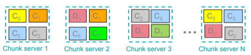
The two other components of DFS (which are not shown in figure) are Master Node and Client library. Master node stores meta data about where files are stored and Client library talks to master to find chunk servers. The other problem in big data computing is moving data around for different computations is computationally expensive. The way to handle this problem is bring computation close to the data. MapReduce is the programming model introduced to handle these problems and DFS is the Storage Infrastructure - File system associated with this programming model.

MapReduce Implementation (centralized)

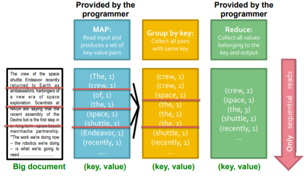
Implementation of MapReduce requires the programmer to write two functions, called Map and Reduce. In brief, a MapReduce computation executes as follows:

1. Some number of Map tasks each are given one or more chunks from a DFS. These Map tasks turn the chunk into a sequence of key-value pairs.

2. The key-value pairs from each Map task are collected by a master controller and sorted by key. The keys are divided among all the Reduce tasks, so all key-value pairs with the same key wind up at the same Reduce task.

3. The Reduce tasks work on one key at a time, and combine all the values associated with that key in some way.

In the diagram bellow, you can see a MapReduce implementation for the word count task. Note that this scheme shows how MapReduce works in a centralized system.

MapReduce Implementation (Parallel)

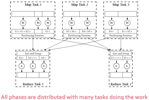
However we are more interested in MapReduce in a computer cluster. In a computer cluster Map and Reduce tasks are running in parallel on multiple nodes. As we mentioned before, same data chunks can appear in different nodes and different Map tasks maybe processing same data chunks. But for the reduce tasks, we want put all key-value pairs with same key to the same reduce task. Here we introduce the Partitioning Function which is just a hash function responsible from this operation. In the figure bellow, you can see the MapReduce reduce diagram in parallel.

MapReduce environment duties:

• Partitioning the input data.
• Scheduling the program’s execution across a set of machines.
• Performing the group by key step.
• Handling machine failures.
• Managing required intermachine communication.

Data Flow

• Input and final output are stored on the DFS.
  • Scheduler tries to schedule map tasks to each chunk server which contains corresponding data chunk.
• Intermediate results are stored on local file system of Map and Reduce workers.

Details of MapReduce Execution

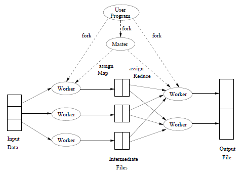
The figure bellow offers an outline of how process, tasks and files interact. Taking advantage of a client library provided by a MapReduce system, the user program forks a Master Controller process and some number of Map workers and Reduce workers. Note that a worker handles either Map tasks or Reduce tasks.

The Master has many responsibilities. One is to create some number of Map tasks and some number of Reduce tasks, these numbers being selected by the user program. These tasks will be assigned to Worker processes by the Master. It is reasonable to create one Map task for every chunk of the input file(s), but we may wish to create fewer Reduce tasks. The reason for limiting the number of Reduce tasks is that it is necessary for each Map task to create an intermediate file for each Reduce task, and if there are too many Reduce tasks the number of intermediate files explodes. The Master keeps track of the status of each Map and Reduce task (idle, executing at a particular Worker, or completed). A Worker process reports to the Master when it finishes a task, and a new task is scheduled by the Master for that Worker process.

Each Map task is assigned one or more chunks of the input file(s) and executes on it the code written by the user. The Map task creates a file for each Reduce task on the local disk of the Worker that executes the Map task. The Master is informed of the location and sizes of each of these files, and the Reduce task for which each is destined. When a Reduce task is assigned by the Master to a Worker process, that task is given all the files that form its input. The Reduce task executes code written by the user and writes its output to a file that is part of the surrounding distributed file system.

Dealing With Failures

• Map worker failure.
  • Map tasks completed or in-progress at worker are rest to idle.
  • Reduce workers are notified when task is rescheduled on another worker.
• Reduce worker failure.
  • Only in-progress tasks are reset to idle.
  • Idle Reduce tasks restarted on other worker(s).
• Master failure.
  • Map reduce task is aborted and client notified.

Refinements

Combiners

• Often a Map task will produce many key-value pairs with same key. We can save time by pre-aggregating values with same key in the mapper.
  • combine(k, list(v1)) -> v2.
  • Combiner is usually same as the reduce function.
  • Works only if reduce function is commutative and associative.

Partition Function

• Want to control how keys get partitioned.
• System uses a default Partition function:
  • hash(key) mod R.
• Sometimes useful to override the hash function.

Algorithms Using MapReduce

The original purpose for which the Google implementation of MapReduce was created was to execute very large matrix-vector multiplications as are needed in the calculation of PageRank.

Matrix-Vector Multiplication by MapReduce

Suppose we have an n x n matrix M, whose element in row i and column j will be denoted m_ij . Suppose we also have a vector v of length n, whose jth element is v_j .

The Map function

Each Map task will operate on a chunk of the matrix M. From each matrix element m_ij it produces the key-value pair (i,m_ijv_j). Thus, all terms of the sum that make up the component x_i of the matrix-vector product will get the same key, i.

The Reduce function

The Reduce function simply sums all the values associated with a given key i. The result will be a pair (i, x_i).

Note that parallelization of matrix multiplication is very crucial at neural net computations.

Natural Join by MapReduce

Natural join is a frequently used operation in relational database system and parallelization of this operation saves enormous computing time. In the figure bellow yo can see the illustration of Natural Join.

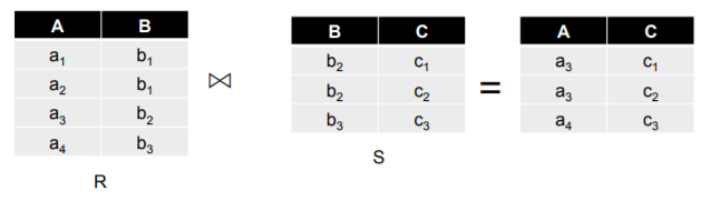
• Use a hash function h from B-values to 1..k
• A map process turns:
  • each input tuple R(a,b) into key-value pair (b, (a,R)).
  • each input tuple S(b,c) into key-value pair (b, (c,S)).
• Map process send each key-value pair with key b to Reduce process h(b).
• Each reduce process matches all the pairs (b, (a,R)) with all (b, (c,S)) and outputs (a,b,c)

Cost Measures for MapReduce Algorithms

Communication Cost

input file size + 2x(sum of the sizes of all files passed from Map process to Reduce process) + the sum of the output sizes of the reduce process.

Elapsed Communication Cost

sum of the largest input + output for any map process + output for any map process

References

• http://web.stanford.edu/class/cs246/
• http://www.mmds.org/#ver21

—- FINDING SIMMILAR DOCUMNETS —-

Shingling of Documents

The most effective way to represent documents as sets, for the purpose of identifying lexically similar documents is to construct from the document the set of short strings that appear within it.

k-Shingles or k-gram

A document is a string of characters. Define a k-shingle for a document to be any substring of length k found within the document. Then, we may associate with each document the set of k-shingles that appear one or more times within that document. Instead of using substrings directly as shingles, we can pick a hash function that maps strings of length k to some number of buckets and treat the resulting bucket number as the shingle. The set representing a document is then the set of integers that are bucket numbers of one or more k-shingles that appear in the document. The result of hashing shingles also called tokens.

Similarity-Preserving Summaries of Sets

Signatures

Sets of shingles are large. Even if we hash them to four bytes each, the space needed to store a set is still roughly four times the space taken by the document. If we have millions of documents, it may well not be possible to store all the shingle-sets in main memory.

Our goal in this section is to replace large sets by much smaller representations called “signatures.” The important property we need for signatures is that we can compare the signatures of two sets and estimate the Jaccard similarity of the underlying sets from the signatures alone.

Minhashing

The signatures we desire to construct for sets are composed of the results of a large number of calculations, say several hundred, each of which is a “minhash” of the characteristic matrix. In this section, we shall learn how a minhash is computed in principle, and in later sections we shall see how a good approximation to the minhash is computed in practice.

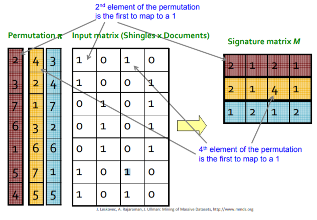
To minhash a set represented by a column of the characteristic matrix, pick a permutation of the rows. The minhash value of any column is the number of the first row, in the permuted order, in which the column has a 1. In the table bellow, you can see an example of minhash table with size 3. The input matrix is a matrix with binary input which has documents in the columns and shingles (tokens) in the rows and this input matrix I, has I_ij =1, if document j contains token i. To calculate the minhash matrix, first we generate 3 different permutation of rows. Lets check the blue permutation. the first row in the blue permutation refers to the sixth row in the input matrix. In the sixth row we see that columns 1 and 3 has inputs 1, so we put the permutation row number (1 in this case) to the first and third columns of the signature vector. the second row in the blue permutation refers to the fourth row in the input matrix. In the fourth row we see that columns 2 and 4 has inputs 1, so we put the permutation row number (2 in this case) to the second and fourth columns of the signature vector. As we filled all columns for the blue permutation, we can proceed to other permutations and fill the column values in the same manner.

Minhashing and Jaccard Similarity

There is a remarkable connection between minhashing and Jaccard similarity of the sets that are minhashed.

The probability that the minhash function for a random permutation of rows produces the same value for two sets equals the Jaccard similarity of those sets.

Computation of Minhas Permutations

It is not feasible to permute a large characteristic matrix explicitly. Even picking a random permutation of millions or billions of rows is time-consuming, and the necessary sorting of the rows would take even more time.

Fortunately, it is possible to simulate the effect of a random permutation by a random hash function that maps row numbers to as many buckets as there are rows. A hash function that maps integers 0, 1, . . . , k −1 to bucket numbers 0 through k−1 typically will map some pairs of integers to the same bucket and leave other buckets unfilled. However, the difference is unimportant as long as k is large and there are not too many collisions. We can maintain the fiction that our hash function h “permutes” row r to position h(r) in the permuted order. Thus, instead of picking n random permutations of rows, we pick n randomly chosen hash functions h1, h2, . . . , hn on the rows. We construct the signature matrix by considering each row in their given order.

Locality Sensitive Hashing (LSH)

The general Idea of LSH is generating a small list of candidate pairs (pairs of elements whose similarity must be evaluated) from the collection of all elements. This is done via “hashing” items several times, in such a way that similar items are more likely to be hashed to the same bucket than dissimilar items are. We then consider any pair that hashed to the same bucket for any of the hashings to be a candidate pair. We check only the candidate pairs for similarity.

LSH for Minhash Signatures

Even though we can use minhashing to compress large documents into small signatures and preserve the expected similarity of any pair of documents, it still may be impossible to find the pairs with greatest similarity efficiently. The reason is that the number of pairs of documents may be too large, even if there are not too many documents. So we refer to the idea of LSH we mentioned above.

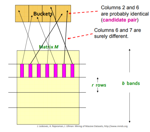
If we have minhash signatures for the items, an effective way to choose the hashings is to divide the signature matrix into b bands consisting of r rows each. For each band, there is a hash function that takes vectors of r integers (the portion of one column within that band) and hashes them to some large number of buckets. We can use the same hash function for all the bands, but we use a separate bucket array for each band, so columns with the same vector in different bands will not hash to the same bucket. In the figure bellow, you can see hash table for a single band in a signature matrix.

Analysis of the Banding Technique

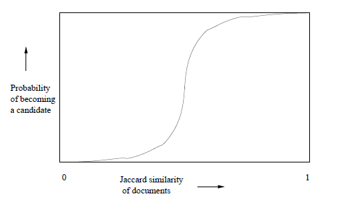
Suppose we use b bands of r rows each, and suppose that a particular pair of documents have Jaccard similarity s. Recall that the probability the minhash signatures for these documents agree in any one particular row of the signature matrix is s. We can calculate the probability that these documents (or rather their signatures) become a candidate pair as follows:

• The probability that the signatures agree in all rows of one particular band is s^r.
• The probability that the signatures disagree in at least one row of a particular band is 1- s^r.
• The probability that the signatures disagree in at least one row of each of the bands is (1- s^r)^b (also the probability of false negatives for s > threshold).
• The probability that the signatures agree in all the rows of at least one band, and therefore become a candidate pair, is 1- (1- s^r)^b. (also the probability of false positives for s < threshold).

It may not be obvious, but regardless of the chosen constants b and r, this function has the form of an S-curve, as suggested in the figure bellow and an approximation for the threshold is (1/b)^1/r. If you want a high recall value, it is better to have high r and low 0

The Theory of Locality-Sensitive Functions

Now, we shall explore other families of functions, besides the minhash functions, that can serve to produce candidate pairs efficiently. These functions can apply to the space of sets and the Jaccard distance, or to another space and/or another distance measure. There are three conditions that we need for a family of functions:

1. They must be more likely to make close pairs be candidate pairs than distant pairs.
2. They must be statistically independent, in the sense that it is possible to estimate the probability that two or more functions will all give a certain response by the product rule for independent events.
3. They must be efficient, in two ways:
   • They must be able to identify candidate pairs in time much less than the time it takes to look at all pairs.
   • They must be combinable to build functions that are better at avoiding false positives and negatives, and the combined functions must also take time that is much less than the number of pairs.

LSH General Formulation

A collection of functions of this form will be called a family of functions. For example, the family of minhash functions, each based on one of the possible permutations of rows of a characteristic matrix, form a family.

Let d1 < d2 be two distances according to some distance measure d. A family F of functions is said to be (d1, d2, p1, p2)-sensitive if for every f in F:

1. If d(x, y) ≤ d1, then the probability that f(x) = f(y) is at least p1.
2. If d(x, y) ≥ d2, then the probability that f(x) = f(y) is at most p2.

LSH Families for Jaccard Distance

The family of minhash functions is a (d1, d2, 1−d1, 1−d2)-sensitive family for any d1 and d2, where 0 ≤ d1 < d2 ≤ 1.

The reason is that if d(x, y) ≤ d1, where d is the Jaccard distance, then SIM(x, y) = 1 − d(x, y) ≥ 1 − d1. But we know that the Jaccard similarity of x and y is equal to the probability that a minhash function will hash x and y to the same value. A similar argument applies to d2 or any distance.

LSH Families for Hamming Distance

Suppose we have a space of d-dimensional vectors, and h(x, y) denotes the Hamming distance between vectors x and y. If we take any one position of the vectors, say the ith position, we can define the function fi(x) to be the ith bit of vector x. Then f_i(x) = f_i(y) if and only if vectors x and y agree in the ith position. Then the probability that f_i(x) = f_i(y) for a randomly chosen i is exactly 1 − h(x, y)/d; i.e., it is the fraction of positions in which x and y agree.

This situation is almost exactly like the one we encountered for minhashing. Thus, the family F consisting of the functions {f1, f2, . . . , fd} is a (d1, d2, 1 − d1/d, 1 − d2/d)-sensitive family of hash functions, for any d1 < d2.

LSH Families for Cosine Distance

Recall that the cosine distance between two vectors is the angle between the vectors. Note that these vectors may be in a space of many dimensions, but they always define a plane, and the angle between them is measured in this plane.

Given two vectors x and y, say f(x) = f(y) if and only if the dot products v_f .x and v_f .y have the same sign. Then F is a locality-sensitive family for the cosine distance. (d1, d2, (180 − d1)/180, (180 − d2)/180)-sensitive family of hash functions. From this basis, we can amplify the family as we wish, just as for the minhash-based family.

Sketches

Instead of choosing a random vector from all possible vectors, it turns out to be sufficiently random if we restrict our choice to vectors whose components are +1 and −1. The dot product of any vector x with a vector v of +1’s and −1’s is formed by adding the components of x where v is +1 and then subtracting the other components of x – those where v is −1. If we pick a collection of random vectors, say v1, v2, . . . , v_n, then we can apply them to an arbitrary vector x by computing v1.x, v2.x, . . . , v_n.x and then replacing any positive value by +1 and any negative value by −1. The result is called the sketch of x.

———– MINING DATA STREAMS ———–

Filtering Data Streams

Bloom Filters

A Bloom filter consists of:

1. An array of n bits, initially all 0’s.
2. A collection of hash functions h1, h2, . . . , hk. Each hash function maps “key” values to n buckets, corresponding to the n bits of the bit-array.
3. A set S of m key values.

The purpose of the Bloom filter is to allow through all stream elements whose keys are in S, while rejecting most of the stream elements whose keys are not in S.

To initialize the bit array, begin with all bits 0. Take each key value in S and hash it using each of the k hash functions. Set to 1 each bit that is hi(K) for some hash function hi and some key value K in S. To test a key K that arrives in the stream, check that all of h1(K), h2(K), . . . , hk(K) are 1’s in the bit-array. If all are 1’s, then let the stream element through. If one or more of these bits are 0, then K could not be in S, so reject the stream element.

Analysis of Bloom Filters

If a key value is in S, then the element will surely pass through the Bloom filter. However, if the key value is not in S, it might still pass. We need to understand how to calculate the probability of a false positive, as a function of n, the bit-array length, m the number of members of S, and k, the number of hash functions.

The model to use is throwing darts at targets. Suppose we have x targets and y darts. Any dart is equally likely to hit any target. After throwing the darts, how many targets can we expect to be hit at least once?

• The probability that a given dart will not hit a given target is (x − 1)/x.

• The probability that none of the y darts will hit a target is ((x − 1)/x)^y. We can write this expression as, (1- 1/x)^x(y/x).

• using the approximation (1-q)^1/q = 1/e, for small q, we conclude that the probability that none of y darts hit a given target is e^-y/x.

• The optimal number of hash functions is (n/m) * ln(2).

Counting Distinct elements in a Stream

Data stream consists of a universe of elements chosen from a set of size N. The problem is maintaining a count of the number of distinct elements seen so far. Unfortunately, we do not have the space to keep the set of elements seen so far. So we need an unbiased estimator for this count. Here we introduce the Flajolet- Martin Algorithm.

Flajolet - Martin Algorithm

• Pick a has function h, that maps each of N elements to at least log₂N bits.
• For each stream element a, let r(a) be the number of trailing zeros in h(a). And R = max_ar(a), over all items a seen so far.
• Estimated number of distinct element is = 2^R.

Analysis of Flajolet - Martin Algorithm

This estimate makes intuitive sense. The probability that a given stream element a has h(a) ending in at least r 0’s is 2^-r. Suppose there are m distinct elements in the stream. Then the probability that none of them has tail length at least r is (1-2^-r)^m. This probability is approximately, e^-m2-r.

1. if m « 2^r, then the probability that we shall find a tail of length at least r approaches 0.
2. if m » 2^r, then the probability that we shall find a tail of length at least r approaches 1.
3. thus 2^R will be always around m.

The problem is that the probability halves when we increase R to R+1, but value doubles. We can use many hash functions h_i. and get many samples of R_i by first sorting all 2^R values. After that;

• Partition your samples into small groups.
• Take the median of groups.
• Then take the average of the medians.

Computing Moments

In this section we consider a generalization of the problem of counting distinct elements in a stream. The problem, called computing “moments,” involves the distribution of frequencies of different elements in the stream. We shall define moments of all orders and concentrate on computing second moments, from which the general algorithm for all moments is a simple extension.

Definition of moments

Suppose a stream consists of elements chosen from a universal set and assume the universal set is ordered. Let m_i be the number of occurrences of the ith element for any i. Then kth moment of the stream is the sum over all i of (m_i)^k.

• 0th moment : number of distinct elements.
• 1st moment : length of the stream.
• 2nd moment : a measure of how uneven the distribution is.

AMS Method

Suppose we do not have enough space to count all the mi’s for all the elements of the stream. We can still estimate the second moment of the stream using a limited amount of space; the more space we use, the more accurate the estimate will be. We compute some number of variables. For each variable X, we store:

1. A particular element of the universal set, which we refer to as X.element.
2. An integer X.value, which is the value of the variable. To determine the value of a variable X, we choose a position in the stream between 1 and n, uniformly and at random. Set X.element to be the element found there, and initialize X.value to 1. As we read the stream, add 1 to X.value each time we encounter another occurrence of X.element .

example:

Suppose the stream is a, b, c, b, d, a, c, d, a, b, d, c, a, a, b. The length of the stream is n = 15. Since a appears 5 times, b appears 4 times, and c and d appear three times each, the second moment for the stream is 5²+4²+3²+3² = 59. Suppose we keep three variables, X1, X2, and X3. Also, assume that at “random” we pick the 3rd, 8th, and 13th positions to define these three variables.

When we reach position 3, we find element c, so we set X1.element = c and X1.value. Position 4 holds b, so we do not change X1. Likewise, nothing happens at positions 5 or 6. At position 7, we see c again, so we set X1.value = 2.

At position 8 we find d, and so set X2.element = d and X2.value = 1. Positions 9 and 10 hold a and b, so they do not affect X1 or X2. Position 11 holds d so we set X2.value = 2, and position 12 holds c so we set X1.value = 3.

At position 13, we find element a, and so set X3.element = a and X3.value = 1. Then, at position 14 we see another a and so set X3.value = 2. Position 15, with element b does not affect any of the variables, so we are done, with final values X1.value = 3 and X2.value = X3.value = 2.

We can derive an estimate of the second moment from any variable X. This estimate is n(2X.value − 1).

—– DIMENSIONALITY REDUCTION —–

Eigenvalues and Eigenvectors of Symmetric Matrixes

Let M be a square matrix. Let λ be a constant and e a nonzero column vector with the same number of rows as M. Then λ is an eigenvalue of M and e is the corresponding eigenvector of M if Me = λe.

Some properties of Symmetric Matrices

1. All eigenvalues of a symmetric matrix are real.
2. If x is a right eigenvector of M wit eigen value λ, x is also a left eigenvector for the same eigenvalue.
3. If M is symmetric, eigenvectors associated to different eigenvalues are mutually orthogonal.
4. Assume V is an orthonormal eigenvector basis for a symmetric matrix M. Then, V^TV=VV^T=I. This also implies V is invertible and its inver is V^T.

Using Eigenvectors for Dimensionality Reduction

From the example we have just worked out, we can see a general principle. If M is a matrix whose rows each represent a point in a Euclidean space with any number of dimensions, we can compute M^TM and compute its eigenpairs. Let E be the matrix whose columns are the eigenvectors, ordered as largest eigenvalue first. Define the matrix L to have the eigenvalues of M^TM along the diagonal, largest first, and 0’s in all other entries. Then, since M^TMe = λe = eλ for each eigenvector e and its corresponding eigenvalue λ, it follows that M^TM = EL.

We observed that ME is the points of M transformed into a new coordinate space. In this space, the first axis (the one corresponding to the largest eigenvalue) is the most significant; formally, the variance of points along that axis is the greatest. The second axis, corresponding to the second eigenpair, is next most significant in the same sense, and the pattern continues for each of the eigenpairs. If we want to transform M to a space with fewer dimensions, then the choice that preserves the most significance is the one that uses the eigenvectors associated with the largest eigenvalues and ignores the other eigenvalues.

Singular Value Decomposition (SVD)

We now take up a second form of matrix analysis that leads to a low-dimensional representation of a high-dimensional matrix. This approach, called singular- value decomposition (SVD), allows an exact representation of any matrix, and also makes it easy to eliminate the less important parts of that representation to produce an approximate representation with any desired number of dimensions.

Definition of SVD

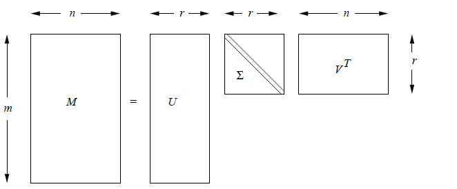
Let M be an m × n matrix, and let the rank of M be r. Recall that the rank of a matrix is the largest number of rows (or equivalently columns) we can choose for which no nonzero linear combination of the rows is the all-zero vector 0 (we say a set of such rows or columns is independent). Then we can find matrices U, Sigma, and V with the following properties:

1. U is an m × r column-orthonormal matrix ; that is, each of its columns is a unit vector and the dot product of any two columns is 0.
2. V is an n × r column-orthonormal matrix.
3. Sigma is a diagonal matrix; that is, all elements not on the main diagonal are 0. The elements of Sigma are called the singular values of M.

Dimensionality Reduction Using SVD

Suppose we want to represent a very large matrix M by its SVD components U, Sigma, and V, but these matrices are also too large to store conveniently. The best way to reduce the dimensionality of the three matrices is to set the smallest of the singular values to zero. If we set the s smallest singular values to 0, then we can also eliminate the corresponding s columns of U and V.

The choice of the lowest singular values to drop when we reduce the number of dimensions can be shown to minimize the root-mean-square error between the original matrix M and its approximation. Since the number of entries is fixed, and the square root is a monotone operation, we can simplify and compare the Frobenius norms of the matrices involved.