Deep Unsupervised Learning
Notes from the Berkley course on deep unsupervised Learning.
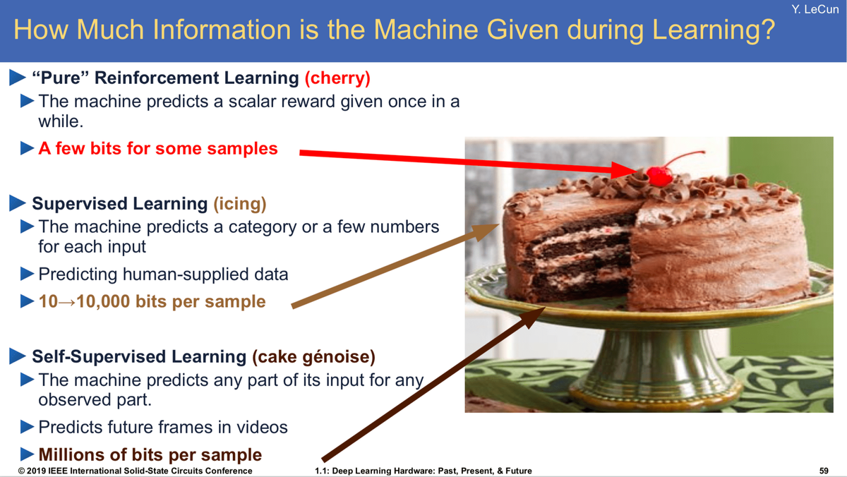 Image credit: Synced
Lecture 1 (Autoregressive Models)
Likelihood-based models
- Problems we’d like to solve: Generating data, compressing data, anomaly detection
- Likelihood-based models estimate the data distribution from some samples from the data distribution
- the aim is to estimate the distribution of complex, high-dimensional data with computational and statistical efficiency.
Generative models
-
Maximum likelihood: given a dataset x(1), …, x(n), find θ by solving the optimization problem.
-
It is equivalent to minimizing KL divergence between the empirical distribution and the model.
How do we solve this optimization problem?
- Stochastic Gradient descent
Why maximum likelihood + SGD? It works with large datasets and is compatible with neural networks.
- Stochastic Gradient descent
Designing The Model
- The key requirement for maximum likelihood + SGD: efficiently compute log p(x) and its gradient.
- pθ —> deep neural network
Autoregressive model
An expressive Bayes net structure with neural network conditional distributions yields an expressive model for p(x) with tractable maximum likelihood training.
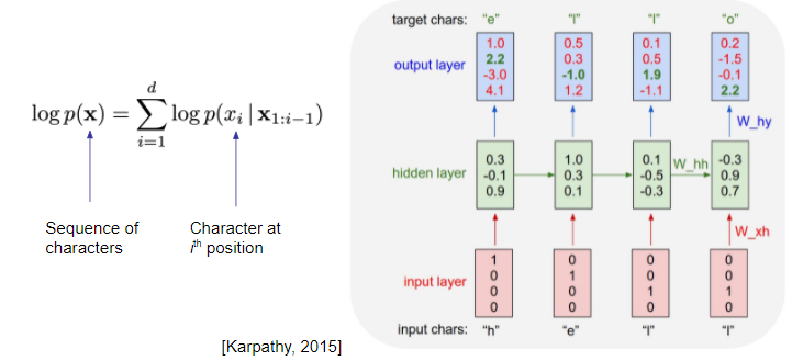
RNN autoregressive models - char-rnn
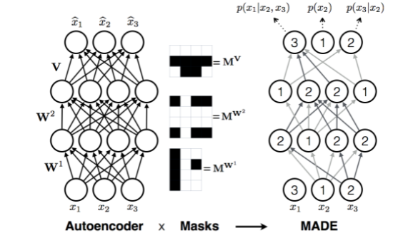
Masking-based autoregressive models
-
Masked Autoencoder for Distribution Estimation (MADE)
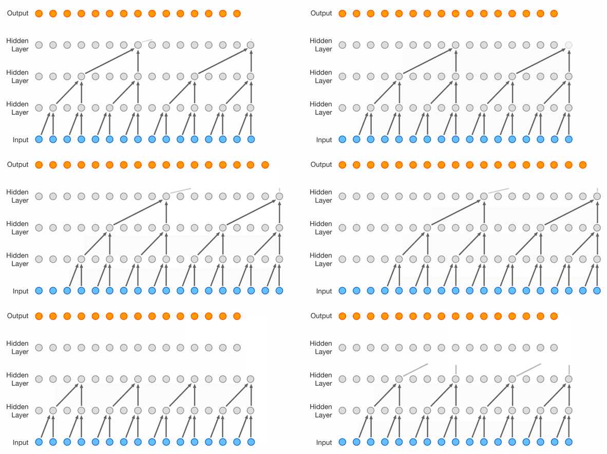
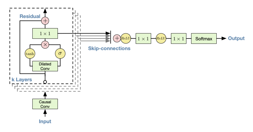
Masked Temporal (1D) Convolution (WaveNet)
Improved receptive field: dilated convolution, with exponential dilation. Better expressivity: Gated Residual blocks, Skip connections.
Masked Spatial (2D) Convolution - PixelCNN
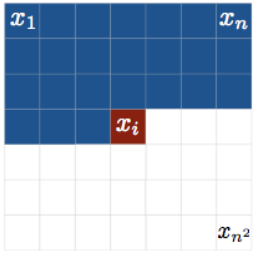
- Images can be flatten into 1D vectors, but they are fundamentally 2D.
- We can use a masked variant of ConvNet to exploit this knowledge.
- First, we impose an autoregressive ordering on 2D images:
PixelCNN
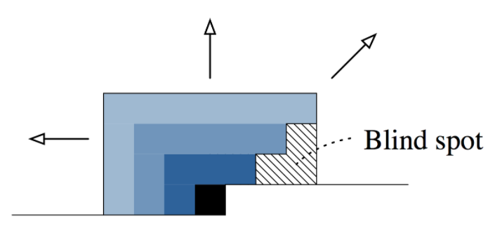
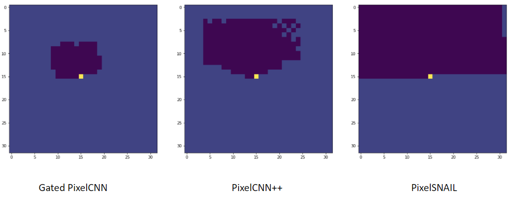
PixelCNN-style masking has one problem: blind spot in the receptive field.
Masked Attention + Convolution
Neural autoregressive models: the good
Best in class modeling performance:
- expressivity - autoregressive factorization is general.
- generalization - meaningful parameter sharing has good inductive bias.
Masked autoregressive models: the bad
-
Sampling each pixel (1 forward pass)
Speedup by breaking the autoregressive pattern
- O(d) -> O(log(d)) by parallelizing within groups {2, 3, 4}.
- Cannot capture dependencies within each group: this is a fine assumption if all pixels in one group are conditionally independent.
- Most often they are not, then you trade expressivity for sampling speed.

Natural Image Manipulation for Autoregressive Models using Fisher Scores
- Main challenge:
- How to get a latent representation from PixelCNN?
- Why hard? The random input happens on a per-pixel sample basis.
- Proposed solution
- Use Fisher score


Lecture 2 (Flow Models)
- How to fit a density $p_Q(x)$ model with continuous $x \in R^n$
- What do we want from this model?
- Good fit to the training data (really, the underlying distribution!)
- For new x, the ability to evaluate $p_\theta (x)$
- Ability to sample from $p_\theta (x)$
- And, ideally, a latent representation that’s meaningful
How to fit a density model?
Option 1: Mixture of Gaussians
Parameters: means and variances of components, mixture weights
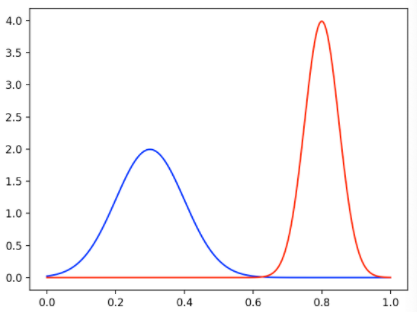
Option 2: General Density Model

- How to ensure proper distribution?

- How to sample?
- Latent representation?
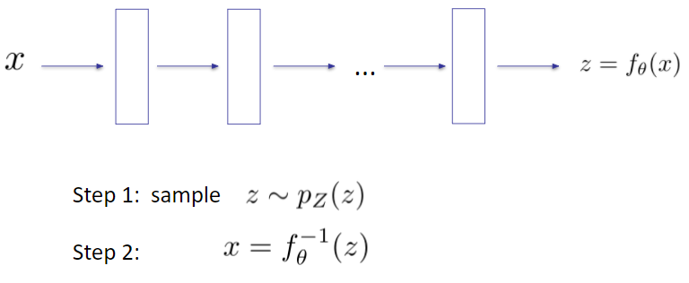
Flows: Main Idea
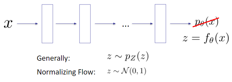
Flows: Training
Change of Variable
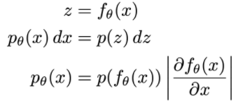
Note: requires invertible & differentiable

assuming we have an expression for , this can be optimized with Stochastic Gradient Descent
Flows: Sampling
2-D Autoregressive Flow

2-D Autoregressive Flow: Face
Architecture: Base distribution: Uniform[0,1]^2 x1: mixture of 5 Gaussians x2: mixture of 5 Gaussians, conditioned on x1

Autoregressive flows
-
How to fit autoregressive flows?
- Map x to z
- Fully parallelizable
-
Notice
- x → z has the same structure as the log likelihood computation of an autoregressive model
- z → x has the same structure as the sampling procedure of an autoregressive model

Inverse autoregressive flows
- The inverse of an autoregressive flow is also a flow, called the inverse autoregressive flow (IAF)
- x → z has the same structure as the sampling in an autoregressive model
- z → x has the same structure as log likelihood computation of an autoregressive model. So, IAF sampling is fast

AF vs IAF
- Autoregressive flow
- Fast evaluation of p(x) for arbitrary x
- Slow sampling
- Inverse autoregressive flow
- Slow evaluation of p(x) for arbitrary x, so training directly by maximum likelihood is slow.
- Fast sampling
- Fast evaluation of p(x) if x is a sample
- There are models (Parallel WaveNet, IAF-VAE) that exploit IAF’s fast sampling.
Change of MANY variables
For , the sampling process f-1 linearly transforms a small cube
to a small parallelepiped
. Probability is conserved:

Intuition: x is likely if it maps to a “large” region in z space
High- Dimensional Flow models: training
Change-of-variables formula lets us compute the density over x:
Train with maximum likelihood:
New key requirement: the Jacobian determinant must be easy to calculate and differentiate!
NICE/RealNVP
- Split variables in half:

- Invertible! Note that $sθ$ and $t_θ$ can be arbitrary neural nets with no restrictions.
- Think of them as data-parameterized elementwise flows.
