Deep Reinforcement Learning
Notes from the UCL course on Reinforcement Learning.
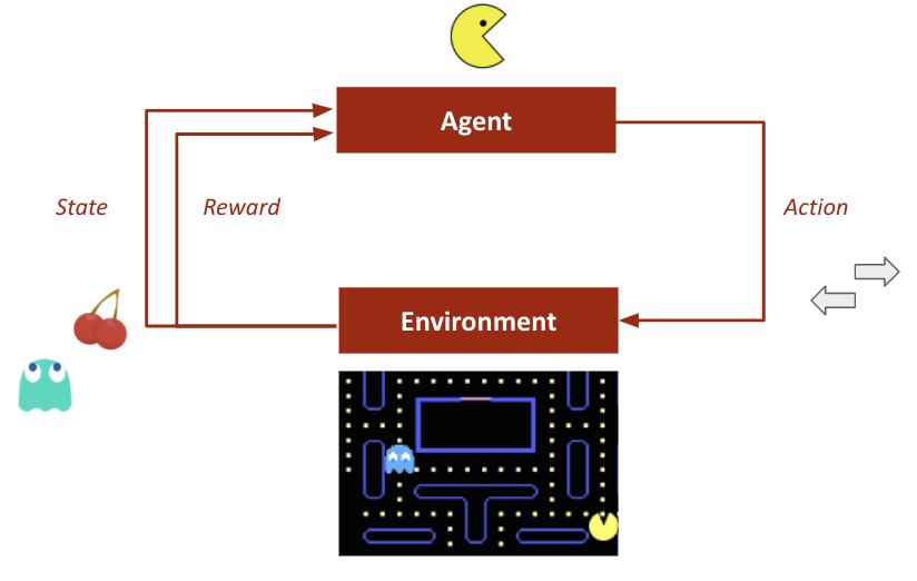 Image credit: Unsplash
LECTURE 1(Introduction to RL)
Characteristic of Reinforcement Learning
- There is no supervisor, only a reward signal.
- Feedback is delayed, not instantaneous.
- Time matters, (sequential, not i.i.d).
- Agent’s actions affects the subsequent data it receives.
Rewards
A reward Rt is a scaler feedback signal indicates how well the agent is doing at step t. The agents job is to maximize the cumulative reward. Reinforcement learning is based on Reward Hypothesis.
Sequential Decision Making
In RL, the actions should be selected to maximize total feature reward. Actions may have long term consequences and rewards maybe delayed. It maybe better to sacrifice immediate reward to gain more long-term reward.
Agent and Environment
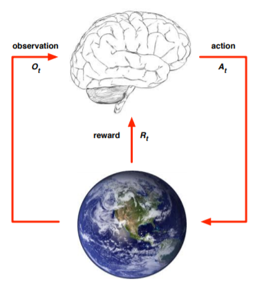
At each time step t the agent:
- Executes Action At.
- Receives observation Ot.
- Receives scaler reward Rt.
At each time step t the environment:
- Receives action At.
- Emits observation Ot+1.
- Emits scaler reward Rt+1
Information State (a.k.a Markov state)
An information state contains all the useful information from history.
Definition
A state St is a Markov if and only if:
P[St+1|St] = P[St+1|S1,…,St]
This means the future is independent of the past given the present.
Fully Observable Environments
The observation at time t is equal to Agent state at time t and the environment state at time t.
Ot = Sta = Ste.
This is a Markov decision process (MDP).
Partially Observable Environments
The agent indirectly observes the environment.
- A robot with camera vision isn’t told its absolute location.
- A trading agent only observes current prices.
- A poker playing agent only observes public cards.
Now, the agent state is not equal to the environment state. Formally, this is a Partially observable Markov decision process (POMDP).
Agent must construct its own state representation Sta, e.g.
- Complete history, Sta = HSt
- Beliefs of environment state.
- Recurrent neural networks.
Major Components of an RL Agent
A RL agent may include one or more of these components.
- Policy: agent’s behaviour function.
- Value function: how good is each state and/or action.
- Model: agent’s representation of the environment.
Policy
- It is a map from state to action, e.g.
- Deterministic Policy
- Stochastic Policy
Value Function
- Value function is a prediction of future reward.
- Used to evaluate the goodness of states.
- And therefore to select between actions.
Model
A model predicts what the environment will do next.
- Transitions model: predicts the next state.
- Reward model : predicts the next reward.
Categorizing RL agents
- Value Based.
- Policy Based.
- Actor Critic.
- Model Free.
- Model Based.
Learning and Planning
Two fundamental problems in sequential decision making:
-
Reinforcement Learning:
- The environment is initially unknown.
- The agent interacts with the environment.
- The agent improves its policy.
-
Planning:
- A model of the environment is known.
- The agent performs computations with its model (without any external interaction)
- The agent improves its policy
Here you can see my Connect4 bot working with a Planning manner and finds the optimal policy with a tree search.
LECTURE 2(MDP)
Markov Process
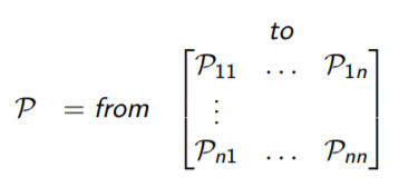
State Transition Matrix
For a Markov state s and successor state s', the state transition probability is defined by,
Pss' = P[St+1 = s' |St = s]
The state transition matrix P defines transition probabilities from all state s to all successor states s'.
Markov Process
A Markov process is a memoryless random process i.e. a sequence of random states S1,S2…Sn with Markov property.
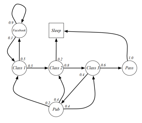
Example :Student Markov Chain
In the figure bellow, you can see the illustration of a student Markov chain :)
Markov Reward Process
A Markov reward process is a Markov chain with values.
Pss' = P[St+1 = s' |St = s]
R is a reward function, Rs = E[Rt+1 |St = s]
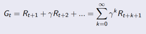
Return
The return Gt is the total discounted reward from time-step t where gamma is the discount factor takes values between 0 and 1. This values immediate reward above delayed reward. Gamma close to 0 leads to ”myopic” evaluation. On the other hand Gamma close to 1 leads to ”far-sighted” evaluation.
Value Functions
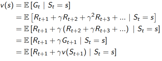
The value function v(s) gives the long term value of state s. The sate value function v(s) of an MRP is the expected return starting from state s.
v(s) = E[Gt |St = s]
Bellman Equation for MRPs
The value function can be decomposed into two parts:
- immediate reward Rt+1
- discounted value of successor state gamma * v(St+1)
Bellman Equation in Matrix Form
The Bellman equation can be expressed concisely using matrices,
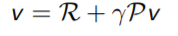
where v is a column vector with one entry per state
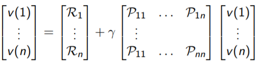
Solving the Bellman Equation
Belllman equation is a linear equation so it can be solved directly. However the computational complexity for is O(n3) for n states so direct solution is only possible for small MRPs. For large MRPs, the iterative methods are:
- Dynamic programming
- Monte - Carlo evaluation
- Temporal Difference learning
Markov Decision Process
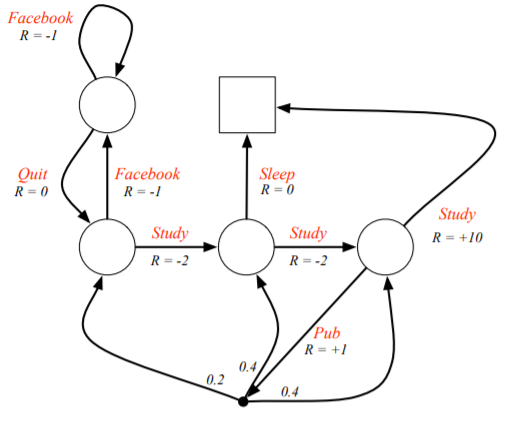
A Markov decision process is a Markov reward process with decisions. It is an environment in which all states are Markov. In the figure bellow, you can see the Student MDP. This time there is no transition probabilities but decisions and rewards. Except going to pub… Once you go to a pub, you can’t make further decisions :)
To make decisions, we need policies.
Policies
A policy π is a distribution over actions given states.
π(a|s) = P [At = a | St = s]
- A policy fully defines the behaviour of an agent.
- MDP policies depend on the current state.
- Policies are stationary, (time independent).
Given an MDP M = <S, A,P, R, γ> and a policy π,
- The state sequence S1, S2, … is a Markov process <S,Pπ>.
- The state and reward sequence S1, R1, S2, … ,s a Markov reward process <S,Pπ,Rπ,γ>.
Value Function
State - Value Function
The state-value function vπ(s) of an MDP is the expected return starting from state s, and then following policy π.
vπ(s) = Eπ [Gt | St = s]
The state-value function can again be decomposed into immediate reward plus discounted value of successor state.
vπ(s) = Eπ [Rt+1 + γvπ(St+1) | St = s]
Action - Value Function
The action-value function qπ(s, a) is the expected return starting from state s, taking action a, and then following policy π.
qπ(s, a) = Eπ [Gt | St = s, At = a]
The action-value function can similarly be decomposed,
qπ(s) = Eπ [Rt+1 + γqπ(St+1,At+1) | St = s, At = a]
Optimal Value Function
- The optimal state-value function v∗(s) is the maximum value function over all policies.
- The optimal action-value function q∗(s, a) is the maximum action-value function over all policies
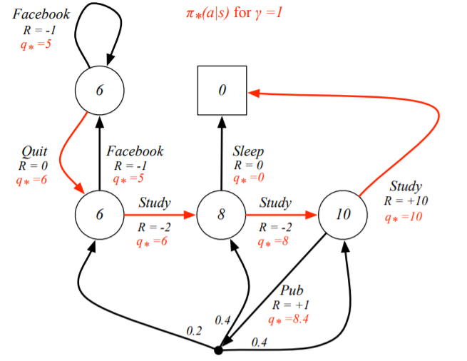
Finding an Optimal Policy
An optimal policy can be found by maximizing over q∗(s, a),
- There is always a deterministic optimal policy for any MDP.
In the figure bellow, the red arcs shows the optimal policy for the student MDP.
Solving the Bellamn Optimality Equation
Bellman optimality equation is non-linear so we introduce some iterative methods such as,
- Value Iteration
- Policy Iteration
- Q-learning
- Sarsa
LECTURE 3(Planning by DP)
Policy Evaluation
- Problem : evaluate a given policy π.
- Solution : iterative application of Bellman expectation backup.
v1 → v2 → … → vπ
Using synchronous backups,
- At each iteration k + 1.
- For all states s ∈ S.
- Update vk+1(s) from vk (s').
- where s' is the successor state of s.
Policy Iteration
Given a policy π,
Evaluate the policy π,
vπ(s) = E[Rt+1 + Rt+2 + … | St = s]
Improve the policy by acting greedily with respect to vπ.
this process of policy iteration always converges to π∗